贝叶斯基本知识点:
先验概率: 基于主观经验或已有的知识推断,对某个随机变量的不确定性的一种猜测。
似然函数: 似然函数是一种关于统计模型参数的函数,即在给定观测值时,关于参数的似然函数等于给定参数后观测值的概率。ps:同时我们可以利用似然函数估计样本的分布参数。
后验概率: 一个随机事件或者一个不确定事件的后验概率是在考虑和给出相关证据或数据后所得到的条件概率。
共轭先验: 在贝叶斯统计中,如果后验分布与先验分布属于同类,则先验分布与后验分布被称为共轭分布,而先验分布被称为似然函数的共轭先验。
利用伯努利随机变量建模页面点击率:
测试两个版本的页面p1,比较两个版本页面到页面P2的点击率。
建立符合属性的模拟数据:
library(bayesAB)

A_binom <- rbinom(250, 1, .25)
B_binom <- rbinom(250, 1, .2)
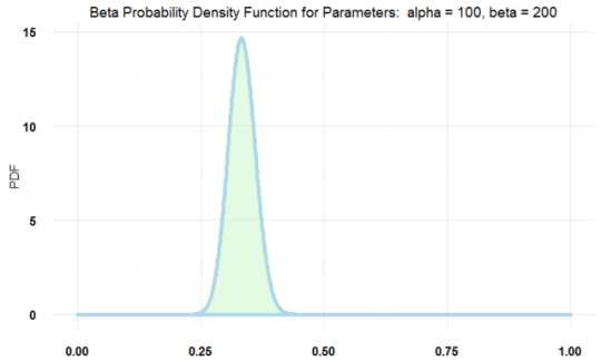
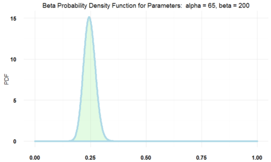
根据以前的经验,设定伯努利分布参数p在0.2到0.3之间。伯努利分布的共轭先验是贝塔分布。(?bayestest查看更多信息):
plotBeta(100, 200) #看起来有点超过0.3了
plotBeta(65, 200) # perfect
利用先验分布拟合:
AB1 <- bayesTest(A_binom, B_binom, priors = c('alpha' = 65, 'beta' = 200), n_samples = 1e5, distribution = 'bernoulli')
bayesTest的结果可以通过print,plot, summary来查看:
print(AB1)

--------------------------------------------
Distribution used: bernoulli
--------------------------------------------
Using data with the following properties:
         [,1] [,2]
Min.    0.000 0.00
1st Qu. 0.000 0.00
Median  0.000 0.00
Mean    0.272 0.26
3rd Qu. 1.000 1.00
Max.    1.000 1.00
--------------------------------------------
Priors used for the calculation:
alpha  beta
   65   200
--------------------------------------------
Calculated posteriors for the following parameters:
Probability
--------------------------------------------
Monte Carlo samples generated per posterior:
[1] 1e+05
summary(AB1)

Quantiles of posteriors for A and B:

$Probability
$Probability$A_probs
       0%       25%       50%       75%      100%
0.1765969 0.2450656 0.2579389 0.2711302 0.3507096

$Probability$B_probs
       0%       25%       50%       75%      100%
0.1735532 0.2394098 0.2521955 0.2651429 0.3352067
--------------------------------------------
P(A > B) by (0)%:
$Probability
[1] 0.58544
--------------------------------------------
Credible Interval on (A - B) / B for interval length(s) (0.9) :
$Probability
        5%        95%
-0.1414135  0.2194684
--------------------------------------------
Posterior Expected Loss for choosing B over A:
$Probability
[1] 0.1099396
plot(AB1)

print输出bayestest的输入,summary输出P((A - B) / B > percentLift)以及在(A - B) / B上的置信区间。plot会画出先验,后验以及蒙特卡洛样例。
利用泊松随机变量建模在某个页面进行交互的次数:
在页面p2上使用者可以进行任何次数的交互,假定每个使用者交互的次数符合泊松分布。依据已有的经验大部分用户进行5到6次的交互。泊松分布的共轭先验是伽马分布。
A_pois <- rpois(250, 6.5)
B_pois <- rpois(250, 5.5)

plotGamma(30, 5) # 5-6 seem likely enough
利用先验分布拟合:
AB2 <- bayesTest(A_pois, B_pois, priors = c('shape' = 30, 'rate' = 5), n_samples = 1e5, distribution = 'poisson')

print(AB2)

--------------------------------------------
Distribution used: poisson
--------------------------------------------
Using data with the following properties:
          [,1]   [,2]
Min.     0.000  0.000
1st Qu.  5.000  4.000
Median   6.000  6.000
Mean     6.556  5.672
3rd Qu.  8.000  7.000
Max.    15.000 14.000
--------------------------------------------
Priors used for the calculation:
shape  rate
   30     5
--------------------------------------------
Calculated posteriors for the following parameters:
Lambda
--------------------------------------------
Monte Carlo samples generated per posterior:
[1] 1e+05
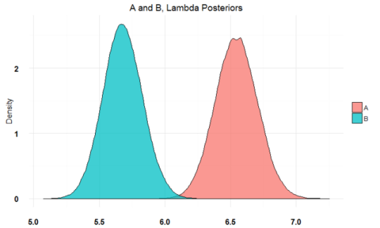
summary(AB2)
Quantiles of posteriors for A and B:
$Lambda
$Lambda$A_lambdas
0% 25% 50% 75% 100%
5.814994 6.435677 6.543340 6.651831 7.250078
$Lambda$B_lambdas
0% 25% 50% 75% 100%
5.076140 5.577516 5.676838 5.778611 6.337962
--------------------------------------------
P(A > B) by (0)%:
$Lambda
[1] 0.99998
--------------------------------------------
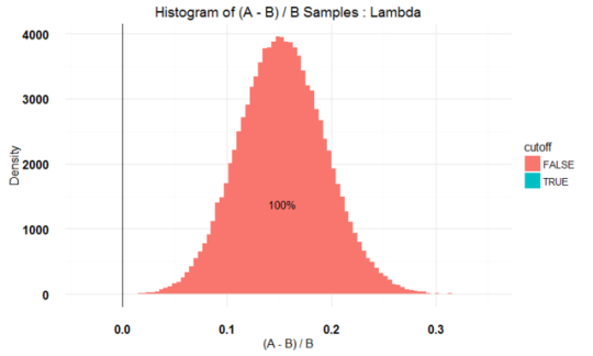
Credible Interval on (A - B) / B for interval length(s) (0.9) :
$Lambda
5% 95%
0.08609353 0.22236109
--------------------------------------------
Posterior Expected Loss for choosing B over A:
$Lambda
[1] 0.0001231939
plot(AB2)
构建联合分布:
bayesAB 能够将不容易参数化的分布分解为一系列容易参数化的分布。例如想test从页面1到页面2的用户在页面2的交互次数。可以根据上面构建的中间分布建立最终分布:
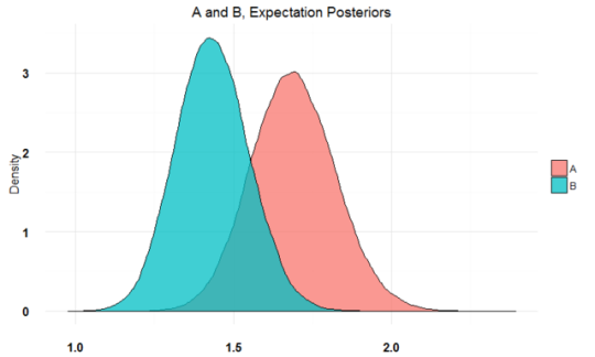
AB3 <- combine(AB1, AB2, f = `*`, params = c('Probability', 'Lambda'), newName = 'Expectation')

# also equivalent with %>% if you like piping
library(magrittr)

AB3 <- AB1 %>%
  combine(AB2, f = `*`, params = c('Probability', 'Lambda'), newName = 'Expectation')
在联合分布中使用乘法,因为对于页面2中泊松分布的每个值都首先要乘以从页面1到页面2的概率。这个结果类似于在页面2的交互的期望值,所以这里取名为Expectation。
print(AB3)

--------------------------------------------
Distribution used: combined
--------------------------------------------
Using data with the following properties:
         [,1]   [,2] [,3]   [,4]
Min.    0.000  0.000 0.00  0.000
1st Qu. 0.000  5.000 0.00  4.000
Median  0.000  6.000 0.00  6.000
Mean    0.272  6.556 0.26  5.672
3rd Qu. 1.000  8.000 1.00  7.000
Max.    1.000 15.000 1.00 14.000
--------------------------------------------
Priors used for the calculation:
[1] "Combined distributions have no priors. Inspect each element separately for details."
--------------------------------------------
Calculated posteriors for the following parameters:
Expectation
--------------------------------------------
Monte Carlo samples generated per posterior:
[1] 1e+05
summary(AB3)

Quantiles of posteriors for A and B:
$Expectation
$Expectation$A
      0%      25%      50%      75%     100%
1.154528 1.599092 1.687873 1.778612 2.391881
$Expectation$B
       0%       25%       50%       75%      100%
0.9774742 1.3544631 1.4312048 1.5099331 1.9430593
--------------------------------------------
P(A > B) by (0)%:
$Expectation
[1] 0.92862
--------------------------------------------
Credible Interval on (A - B) / B for interval length(s) (0.9) :
$Expectation
         5%         95%
-0.01983823  0.41881674
--------------------------------------------
Posterior Expected Loss for choosing B over A:
$Expectation
[1] 0.1132771
plot(AB3)