完整的代码及运行过程在GitHub上
导入需要使用的R包:
画图:
library(gridExtra)
library(grid)
library(ggplot2)
数据处理:
library(data.table)
library(dplyr)
分类变量变为数值变量:
library(dummies)
数据预处理及模型创建:
library(caret)
读入数据并做简单查看:
train_data <- read.csv(file.choose())
查看数据维度和变量种类:
dim(train_data)
[1] 550068     12

str(train_data)
'data.frame':	550068 obs. of  15 variables:
 $ User_ID                   : int  1000001 1000001 1000001 1000001 1000002 1000003 1000004 1000004 1000004 1000005 ...
 $ Product_ID                : Factor w/ 3631 levels "P00000142","P00000242",..: 673 2377 853 829 2735 1832 1746 3321 3605 2632 ...
 $ Gender                    : Factor w/ 2 levels "F","M": 1 1 1 1 2 2 2 2 2 2 ...
 $ Age                       : Factor w/ 7 levels "0-17","18-25",..: 1 1 1 1 7 3 5 5 5 3 ...
 $ Occupation                : int  10 10 10 10 16 15 7 7 7 20 ...
 $ City_Category             : Factor w/ 3 levels "A","B","C": 1 1 1 1 3 1 2 2 2 1 ...
 $ Stay_In_Current_City_Years: Factor w/ 5 levels "0","1","2","3",..: 3 3 3 3 5 4 3 3 3 2 ...
 $ Marital_Status            : int  0 0 0 0 0 0 1 1 1 1 ...
 $ Product_Category_1        : int  3 1 12 12 8 1 1 1 1 8 ...
 $ Product_Category_2        : int  NA 6 NA 14 NA 2 8 15 16 NA ...
 $ Product_Category_3        : int  NA 14 NA NA NA NA 17 NA NA NA ...
 $ Purchase                  : int  8370 15200 1422 1057 7969 15227 19215 15854 15686 7871 ...
我们看到变量除了目标变量外其他全部都是分类变量,且部分变量存在缺失值。
查看数据是否有缺失值及其缺失项
#查看数据完整例子的数目与数据行数相比较,如果小于数据行数即表示存在缺失项
sum(complete.cases(train_data))
[1] 166821

#查看具体的缺失项的变量
colSums(is.na(train_data))
通过这两个函数可以发现在Product_Category_2, Product_Category_3中存在大量缺失值。
单变量分析
由于各变量全部都是分类变量,我们主要看一下各变量的的类别占比。
prop.table(table(train_data$Gender))
        F         M
0.2468949 0.7531051

prop.table(table(train_data$Marital_Status))
       0        1
0.590347 0.409653

prop.table(table(train_data$City_Category))
        A         B         C
0.2685486 0.4202626 0.3111888

prop.table(table(train_data$Stay_In_Current_City_Years))
        0         1         2         3        4+
0.1352524 0.3523583 0.1851371 0.1732240 0.1540282

prop.table(table(train_data$Age))
0-17      18-25      26-35      36-45      46-50      51-55        55+
0.02745479 0.18117760 0.39919974 0.19999891 0.08308246 0.06999316 0.03909335

prop.table(table(train_data$Occupation))
prop.table(table(train_data$Product_Category_1))

prop.table(table(train_data$Product_Category_2, exclude = NULL))
prop.table(table(train_data$Product_Category_3, exclude = NULL))
从上面可以看到男性用户远远高于女性用户,未婚用户略高于已婚,B城用户更高一些,当前城市居住一年期用户更多,同时我们发现用户年龄主要集中在18岁到45之间。到这其实可以对此公司的用户属性进行一些猜测以便于指导后面的双变量分析,例如新到一个城市单身男性更容易接受此类的产品的猜测。
注:这份数据很可能是有规律的抽取的,所以目前所做的假设是基于数据是完整的或能代表整体的随机性数据。
基于前面的单变量分析进行变量创建
train_first <- train_data
将Gender中的F和M变为0和1:
train_first$Gender <- ifelse(train_first$Gender=='F', 0, 1)
由于City_Category, Stay_In_Current_City_Years类别分布相差不大且类别数目不多,对它们创建虚拟变量。
train_first <- dummy.data.frame(train_first, names = c("City_Category", "Stay_In_Current_City_Years"), sep = "_")
用Age,Occupation, Product_Category_1, Product_Category_2,Product_Category_3中类别的数目代替类别。
train_first <- data.table(train_first)
train_first[, Age_Count := .N, by = Age]
train_first[, Occupation_Count := .N, by = Occupation]
train_first[, Product_Category_1_Count := .N, by = Product_Category_1]
train_first[, Product_Category_2_Count := .N, by = Product_Category_2]
train_first[, Product_Category_3_Count := .N, by = Product_Category_3]
去除不需要的变量
train_first[, Purchase_add := Purchase]
train_first <- subset(train_first, select = -c(Purchase, Age, Occupation, Product_Category_1,Product_Category_2, Product_Category_3))
dim(train_first)
[1] 550068     18
str(train_first)
Classes ‘data.table’ and 'data.frame':	550068 obs. of  18 variables:
 $ User_ID                      : int  1000001 1000001 1000001 1000001 1000002 1000003 1000004 1000004 1000004 1000005 ...
 $ Product_ID                   : Factor w/ 3631 levels "P00000142","P00000242",..: 673 2377 853 829 2735 1832 1746 3321 3605 2632 ...
 $ Gender                       : num  0 0 0 0 1 1 1 1 1 1 ...
 $ City_Category_A              : int  1 1 1 1 0 1 0 0 0 1 ...
 $ City_Category_B              : int  0 0 0 0 0 0 1 1 1 0 ...
 $ City_Category_C              : int  0 0 0 0 1 0 0 0 0 0 ...
 $ Stay_In_Current_City_Years_0 : int  0 0 0 0 0 0 0 0 0 0 ...
 $ Stay_In_Current_City_Years_1 : int  0 0 0 0 0 0 0 0 0 1 ...
 $ Stay_In_Current_City_Years_2 : int  1 1 1 1 0 0 1 1 1 0 ...
 $ Stay_In_Current_City_Years_3 : int  0 0 0 0 0 1 0 0 0 0 ...
 $ Stay_In_Current_City_Years_4+: int  0 0 0 0 1 0 0 0 0 0 ...
 $ Marital_Status               : int  0 0 0 0 0 0 1 1 1 1 ...
 $ Age_Count                    : int  15102 15102 15102 15102 21504 219587 45701 45701 45701 219587 ...
 $ Occupation_Count             : int  12930 12930 12930 12930 25371 12165 59133 59133 59133 33562 ...
 $ Product_Category_1_Count     : int  20213 140378 3947 3947 113925 140378 140378 140378 140378 113925 ...
 $ Product_Category_2_Count     : int  173638 16466 173638 55108 173638 49217 64088 37855 43255 173638 ...
 $ Product_Category_3_Count     : int  383247 18428 383247 383247 383247 383247 16702 383247 383247 383247 ...
 $ Purchase_add                 : int  8370 15200 1422 1057 7969 15227 19215 15854 15686 7871 ...
 - attr(*, ".internal.selfref")=<externalptr>
对变量进行线性回归建模
对变量进行归一化处理
train_first <- data.frame(train_first)
newdata <- train_first[ ,3:17]
preProc <- preProcess(newdata)
newdata_pre <- predict(preProc, newdata)
train_pre <- data.frame(newdata_pre, Purchase=train_first$Purchase_add)
lm建模
lm_model <- lm(Purchase~., data=train_pre)
summary(lm_model)

Residual standard error: 4730 on 550054 degrees of freedom
Multiple R-squared:  0.1135,	Adjusted R-squared:  0.1135
F-statistic:  5416 on 13 and 550054 DF,  p-value: < 2.2e-16
和直接用均值做预测相比较
train_mean <- train_data$Purchase
train_mean <- data.table(train_mean)
train_mean[, Purchase_mean := mean(train_mean)]
sqrt(sum( (train_mean$train_mean - train_mean$Purchase_mean)^2 , na.rm = TRUE ) / nrow(train_mean) )
[1] 5023.061
lm模型只比均值预测好一点,考虑添加新变量。
添加新变量
查看Purchase目标变量
purchase_plot <- ggplot(train_data, aes(Purchase))+geom_area(stat = "bin")
purchase_plot
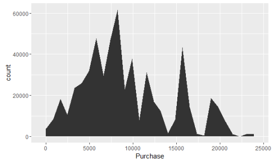
可以看到Purchase呈分段式分布,由几个小高峰组成。
查看Purchase与各变量的关系
年龄与购买金额

居住地与购买金额

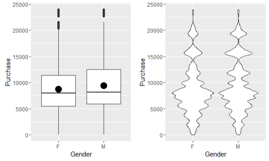
性别与购买金额
是否结婚与购买金额

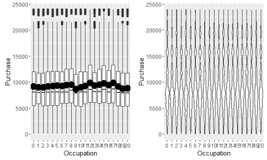
职业与购买金额
居住年限与购买金额

产品种类与购买金额

对User_ID和Product_ID去重
length(unique(train_data$User_ID))
[1] 5891
length(unique(train_data$Product_ID))
[1] 3631
据此创建额外变量
train_first <- data.table(train_first)
train_first[, User_Count := .N, by = User_ID]
train_first[, Product_Count := .N, by = Product_ID]

train_first[, Mean_Purchase_Product := mean(Purchase_add), by = Product_ID]
train_first[, Mean_Purchase_User := mean(Purchase_add), by = User_ID]

train_first[, Purchase := Purchase_add]
train_first <- subset(train_first, select = -c(Purchase_add))
重新lm建模
train_first <- subset(train_first, select = -c(City_Category_C, Stay_In_Current_City_Years_4.))
train_first <- data.frame(train_first)
newdata <- train_first[ ,3:19]
preProc <- preProcess(newdata)
newdata_pre <- predict(preProc, newdata)
train_pre <- data.frame(newdata_pre, Purchase=train_first$Purchase)
lm_model <- lm(Purchase~., data=train_pre)
summary(lm_model)

Residual standard error: 2554 on 550050 degrees of freedom
Multiple R-squared:  0.7415,	Adjusted R-squared:  0.7415
F-statistic: 9.283e+04 on 17 and 550050 DF,  p-value: < 2.2e-16
对模型进行检验
#检查自相关
library(lmtest)
dwtest(lm_model)

	Durbin-Watson test

data:  lm_model
DW = 1.8359, p-value < 2.2e-16
alternative hypothesis: true autocorrelation is greater than 0

#检查多重共线性,需要将变量中的City_Category_C 和 Stay_In_Current_City_Years_4.删掉后重新建模。
library(car)
vif(lm_model)
使用caret包中的train建模
source('D:/log-practice/xgboost.R')
ctrl <- trainControl(method = "repeatedcv", number = 5)
#这里每次训练两个参数,最后得到
xgbgrid <- expand.grid(eta=0.26, gamma=0.1, max_depth=10,
                       min_child_weight=11, max_delta_step=0, subsample=1,
                       colsample_bytree=1, colsample_bylevel = 1, lambda=0.05,
                       alpha=0, scale_pos_weight = 1, nrounds=80, eval_metric='rmse',
                       objective="reg:linear")
xgb_model <- train(train[,3:19], train[,20], method = xgboost,  tuneGrid=xgbgrid, trControl=ctrl)
Purchase <- predict(xgb_model, test[, 3:19])
result_sub <- data.frame(User_ID=test$User_ID, Product_ID=test$Product_ID, Purchase=Purchase)
write.csv(result_sub, file = 'D:/data_practice_1/result_sub.csv', row.names = FALSE)
